I’m a big fan of Flightradar24 and using it to see planes flying ahead made me wonder, is there an open source way of replicating it? I came across this post by @geodose, which shows how to use the OpenSky Network to do just that, using QGIS to refresh the view of a constantly-updating .csv file of live flight data. There are other ways to go about this, of course – an RShiny/leaflet approach would be a good solution but it’s a bit more work to set up and it’s fun to try new things. On that note, let’s start with the end result, then get into the nitty gritty:
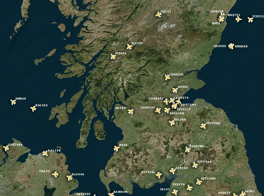
The finished result: 5 minutes of OpenSky data auto-rendering in QGIS (sped up ~7.5x)
Their approach was to call the OpenSky API in Python, whereas I wanted a solution in R. There are some R-based wrappers on the OpenSky website, one of which is the openSkies library [manual here], but using the API it was simpler just to use that as a URL to bring json data into R and go from there. The jsonlite package did the heavy (/light) lifting, then it was a matter of running the script at regular intervals…
Without an account, the OpenSky API allows calls every 10 seconds, which was easily enough for this. In order to constantly refresh the output .csv with live data, I followed this guide on scheduling using the later package by @xieyihui.
All of that put together gives the following R code:
library(jsonlite)

library(later)

wd <- paste0(dirname(rstudioapi::getSourceEditorContext()$path),"/") # if not running in RStudio, set wd to directory of this script, e.g. wd <- 'C:/Dir/'
checkPlane = function(interval = 10) {
json <- jsonlite::fromJSON("https://opensky-network.org/api/states/all?lamin=54.301701&lomin=-8.013080&lamax=60.982102&lomax=-0.493414")
json_df <- as.data.frame(json$states)
colnames(json_df) <- c("icao24","callsign","origin_country","time_position","last_contact","longitude","latitude","baro_altitude","on_ground","velocity","true_track","vertical_rate","sensors","geo_altitude","squawk","spi","position_source")
json_df[,c(4:8,10:14,16,17)] <- lapply(json_df[,c(4:8,10:14,16,17)],as.numeric)
write.csv(json_df,paste0(wd,"current_planes.csv"))
later::later(checkPlane, interval)
}
checkPlane()
Now we’ve got the live data being output every 10 seconds, we’re back to geodose’s tutorial to set up QGIS to read it in. You can follow the steps in that guide, but it starts off just reading in the .csv and styling it. The key elements to get the flight data working how we want are i) setting the symbol rotation to read in the ‘true_track’ attribute (the heading of the plane) and ii) getting QGIS to re-render the input data every 10 seconds, both of which are shown below [images edited from geodose]:
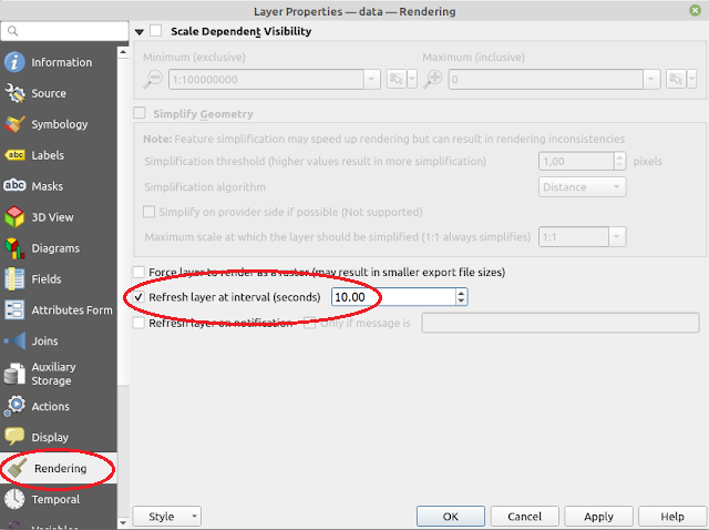
Setting a rendering refresh interval in QGIS
You’ll notice from the gif above that not everything looks perfect with the ‘true_track’ data. The headings occassionally go awry, but for a free and open source dataset, it’s definitely good enough.
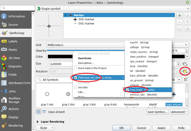
Setting symbol rotation to the ‘true_track’ attribute